Fast dynamic area exclusion in Valhalla

One of the big pros of Valhalla is that it lets you tweak requests at runtime, without needing to rebuild the entire graph from scratch. In Valhalla, we call this philosophy dynamic costing, and it lets us do a lot of cool things. One such thing that Valhalla has been capable of for some time is to let the user pass a list of polygons and avoid the edges intersecting with these in path finding. In this blog post, I want to show you how we have recently significantly sped this avoiding mechanism up so that you can now avoid areas large in size, number, or complexity.

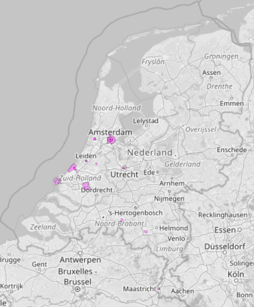
Let’s look at an example: say you want to avoid driving through low emission zones. Valhalla does not currently know about these zones, and so it will happily route you through one. But you, the user, can just pull the geometries of these zones and pass them to Valhalla as exclude_polygons, and it will ignore all intersecting edges during path finding. Take the Dutch low emission zones (milieuzones) from the NDW as an example. It’s a set of 42 polygons rich in detail, spread across the country (though the large ones are mostly in the Randstad):

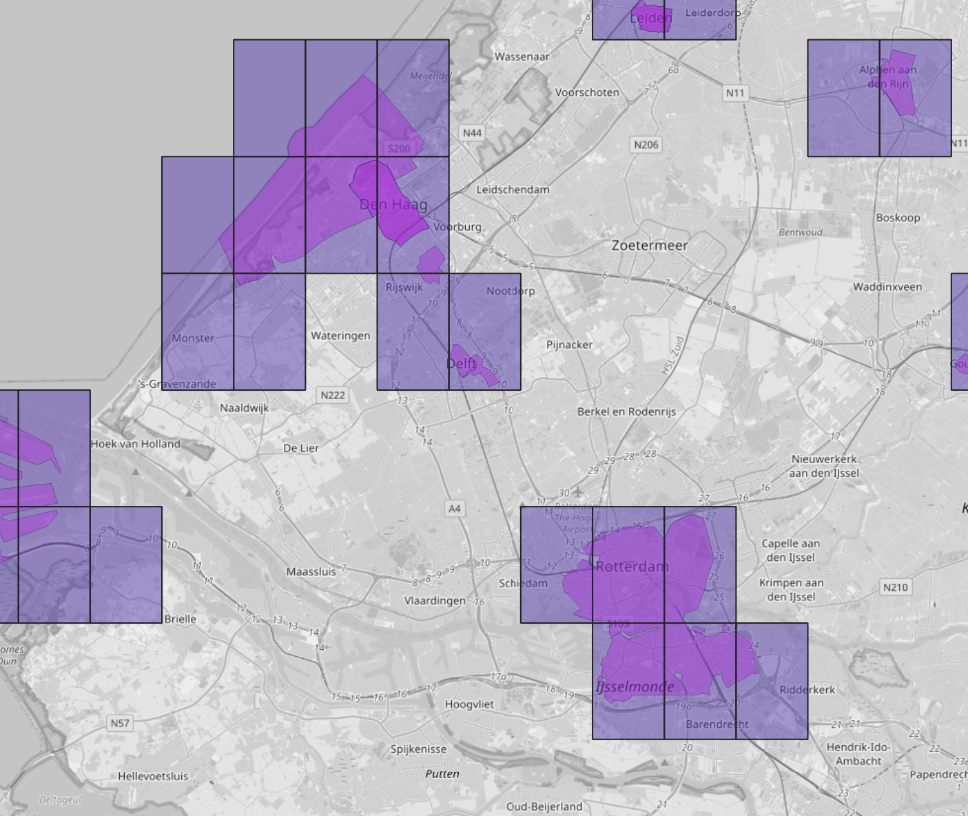
Up until recently, Valhalla’s implementation worked well for a few small polygons with low detail, but it choked on large numbers of polygons, polygons with large areas and highly detailed polygons. So let’s say we wanted to pass all 42 low emission zones in the Netherlands to Valhalla. What Valhalla then used to do was identify the edge bins that intersect each polygon’s boundary (a bin is a 0.05x0.05° rectangle containing intersecting edge identifiers, and acts as Valhalla’s coarse spatial index; that’s roughly 5.6 km at the equator) and do a simple intersect operation between each edge and each polygon. This is very slow, because this means the polygon search runs in O(n*m) time, where n is the total number of vertices across all polygons, and m the total number of edge shape segments in boundary-intersecting bins. Looking at all the bins we’ve just intersected, you can immediately tell why this is bad news: we have to perform this expensive operation against every single edge in Amsterdam, Rotterdam, Den Haag, and more cities… gulp.

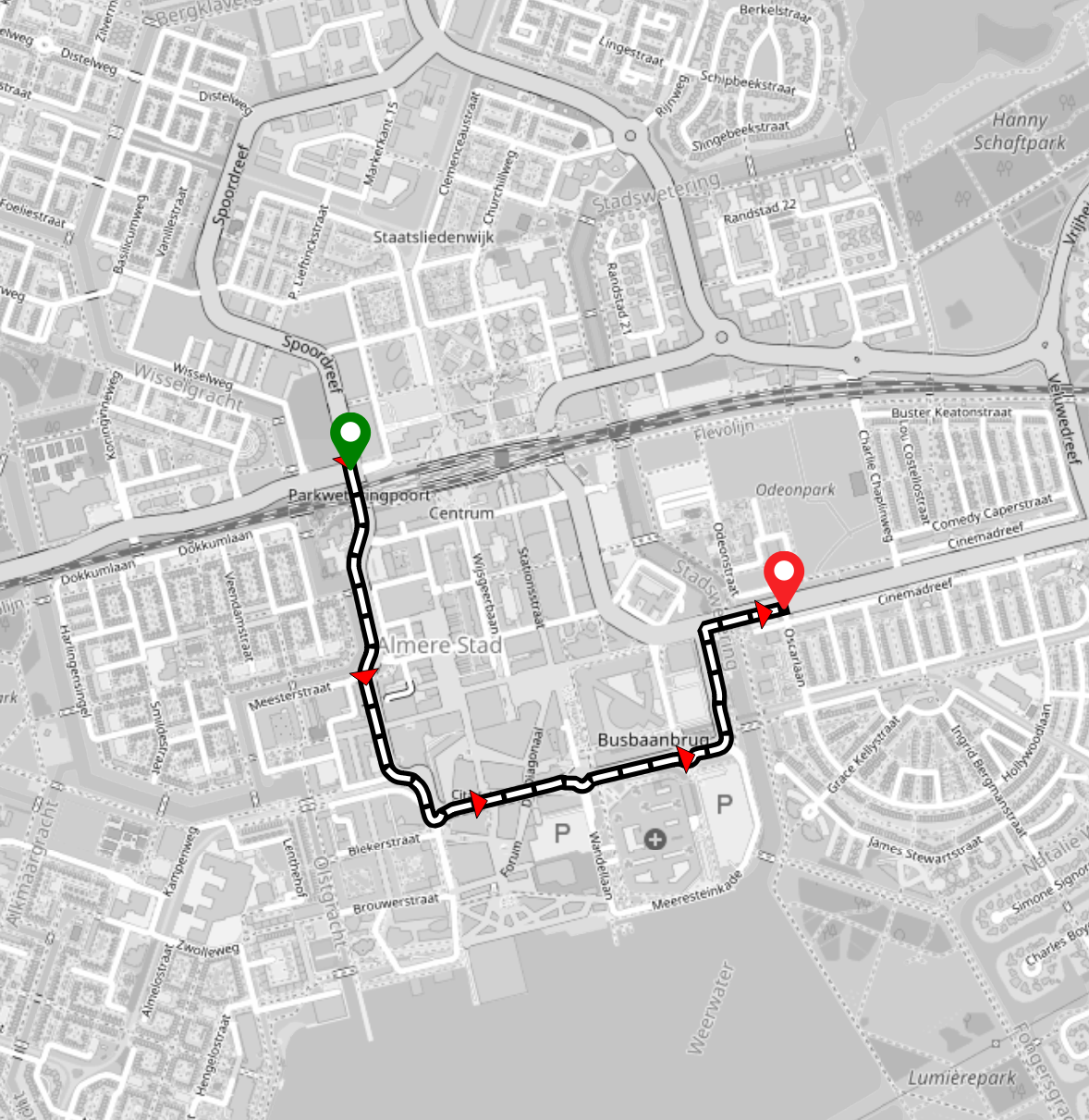
Well, let’s try it out anyway! I pick a short route from one side of Almere’s city center to the other to illustrate the mechanism. The default car route goes straight through the low emission zone:

If we now plug in the low emission zones into the exclude_polygons request parameter, the low emission zone is avoided:

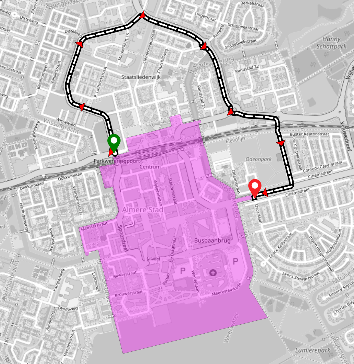
But we don’t get this result immediately. On my machine, the local Valhalla service takes 32 seconds to respond with a route. 32 seconds is of course prohibitively expensive for a routing request. A normal duration for a route request would most likely fall in the 15-300 millisecond range, depending on the exact request, so this takes about 100-2000 times longer than what’s considered a normal route request.

How to make this faster

Bounding geometries

Yes, if you have been reading my blog, you may have already guessed it. Valhalla’s spatial index on the edges recently got better through the use of minimum bounding circles, and we can of course use them here as well. I won’t explain anything about the details here, but you can go read everything about the bounding circles here. What I will say is that we can use the bounding circles to quickly reject edges that are in our 0.05x0.05° bin but nowhere near our input polygons. On the other hand, we can also quickly create a bounding box for each polygon, and speed up this early rejection by making it a very cheap circle-in-rectangle check.

R-Trees

The bounding geometries get us very far, especially for small geometries that only cover small parts of a bin. But looking back at some of the zones, we see that a lot of them cover more than 50% of a single bin’s area. Our cheap rejection won’t work, and Valhalla will have to look at the geometries in detail. Since we will have to perform a lot of intersection tests on each polygon, it could be beneficial to preprocess them once so these repeated operations become cheaper and the preprocessing gets amortized. One way to do this is to construct an r-tree. R-trees are tree data structures that, once constructed, let you quickly filter nearby geometries given a point or a rectangle. Inside, they are just bounding boxes organized hierarchically, grouped in a way that nearby bounding boxes fall into the same group. There are a lot of r-tree implementations out there, but a particularly popular one is called flatbush, originally developed for the browser by Volodymyr Agafonkin. These days, there are plenty of other implementations, and luckily, there is a well maintained C++ one. If you want to read more about how it works and what Hilbert curves have to do with it, I recommend this blog post.

Back to our polygon search though: when performing the intersect, we are interested in looking at as few polygon segments as necessary. So constructing an r-tree per polygon, indexing each of its segments can let us find the segments that are near an edge, filtering out most of a polygon’s segments. Constructing these is relatively inexpensive, especially compared to the hundreds of thousands of intersection checks our search algorithm is currently doing. For reference, this is what the r-tree for Almere’s low emission zone looks like:

The top-level bounding box is the root, which must fit all of its children bounding boxes. The bounding boxes one level deeper again must contain all their children and so on. Bounding boxes on the same level can (and probably will) overlap as you can see on level 2.

So given an edge shape, we form its bounding box and walk the tree from the root down. If a bounding box does not intersect with our edge’s bounding box, we know that none of its children intersect our edge’s bounding box either, so we quickly discard most segments indexed by the tree.

Point-in-polygon

So with our r-tree filter, we can really quickly determine which edges intersect our polygon boundary. But we’re not just interested in the ones crossing the boundary, we also need to know which ones are entirely inside. Once we know an edge does not cross the boundary, there are only two possible relationships left: either the edge lies fully inside the polygon, or it’s fully outside. We can choose any of the edge’s shape points and perform a simple point-in-polygon check to find out. Valhalla has a function for that, which implements the winding number algorithm. It suffers from the problem that we want to get rid of though: it requires looping over all of a polygon’s segments to be able to tell whether a point is inside a polygon, and our r-tree won’t help. Luckily, there is an algorithm that allows us to leverage the r-tree, and it’s called the ray casting algorithm. In short, it can tell whether a point is inside a given polygon by projecting a horizontal ray from the point and counting the intersecting polygon segments. An even count means the point is outside the polygon, an odd count means it’s inside. We only care about polygon segments the ray can reach, which is where our r-tree shines again!

So, how much faster is it?

Plugging our low emission zone polygons into the same request as before, it now takes Valhalla 280 milliseconds to complete the request, which constitutes a ~110x speed up compared to before! That is a significant improvement, placing our example request back into “normal” territory. The number of segments and the total polygon count are no longer bottlenecks in the polygon avoidance. The new bottleneck is now the number of intersected edges: in order to quickly tell whether an edge is even allowed, we keep an in memory hash set of edge IDs to check against during path finding. For large polygons (e.g. an entire mid-sized country), this hash set quickly grows in size, causing cache misses that make lookups slow as the area grows. But one bottleneck at a time.

Further reading

• Valhalla’s documentation for exclude_polygons
• The pull request