The good thing about joining an open source project is that you don’t have to start from scratch. The bad thing about it is that you can’t start from scratch: often, you are limited by what’s been done already. But those limits can also present great opportunities to work on unique problems requiring unique solutions.

In this post, I want to write about my endeavor to speed up Valhalla’s spatial search by improving the spatial index on its graph edges. This started as a conversation I had with Kevin Kreiser about two years ago, about making Valhalla’s path finding around excluded areas faster. He said he’d had an idea for an improved spatial index a while ago, with the goal to speed up the location search, and so I was immediately hooked.

It took me a good amount of experiments (both successful and failed ones), spanning almost two years, working on it here and there, whenever I had some spare time. It ended up making me really comfortable with Valhalla’s concepts and vast code base, because it touched on so many aspects: graph tile building, computational geometry, and the entirety of Valhalla’s location search module. But let’s move through this step by step.

What’s a spatial index, anyway?

Broadly speaking, a spatial index is a way to hierarchically cluster spatial features into groups of nearby features, so that when you want to, for example, find all features within a given distance from a known point, you don’t have to go check each and every feature in your data set; the spatial index helps you quickly find the relevant features. People have thought and written about all kinds of spatial indices for decades, so I will leave it at this broad definition and kindly direct you to the search engine of your choice if you want to know more about the topic.

What does Valhalla’s spatial indexing look like?

Let’s start by looking at a common scenario for any routing software: a user wants to know the best path from point A to point B. The routing software receives two coordinate pairs and, before being able to compute any path, needs to find the nearest viable roads for each point.

Now, the naive approach would be to go through each road segment (referred to from here on as an edge) in the road network (referred to from here on as a graph) and measure the distance from the input points to the closest point on the edge. Except the graph contains every edge in the entire world, and distance measurements aren’t computationally cheap (one could argue that nothing is computationally cheap if you have to do it ~2 billion times).

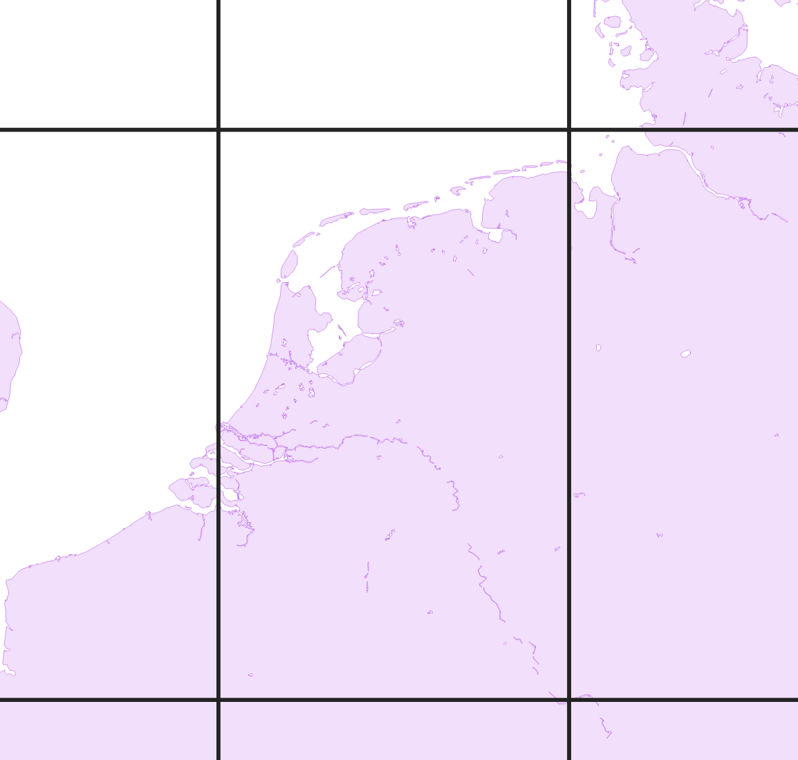
Luckily, the way Valhalla structures its graph makes it easy to do something bit cleverer. It chops up the graph in tiles, which are sets of squares that cover earth’s surface (in reality, tiles are more like hyperbolic trapezoids, but that doesn’t really matter in this context, just throwing a bone to the fuming readers of r/mapporncirclejerk). The world’s road network is first divided into a three-piece hierarchy of roads: level 0 (the “highest”) contains motorways, level 1 arterial roads, and level 2 the rest. Since the higher levels contain fewer roads, their tile sizes can be bigger:

This helps us a great deal: it lets us instantly discard most of the world’s tiles. But now we’re still forced to look at all the edges in tiles from all three hierarchy levels that are near our input points. On level 0, we’d have to look at basically every edge in the entire country, since the spatial resolution is coarsest at that level. And we haven’t even talked about edges that run through more than one tile: edges are stored in the tile they start in, so we might miss those if we just search in tiles that the input location intersects.

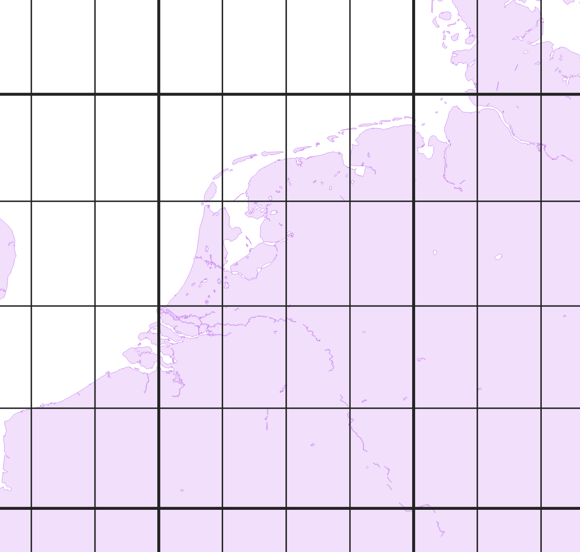
Luckily, Valhalla has another trick up its sleeve: at level 2, tiles are cut up further into sub-tiles, also called bins: these 5x5 squares, each with a resolution of 0.05°x0.05° (roughly 5.6km at the equator). For each bin, we store a list of edges from any level that intersect it, and store those in the tile.

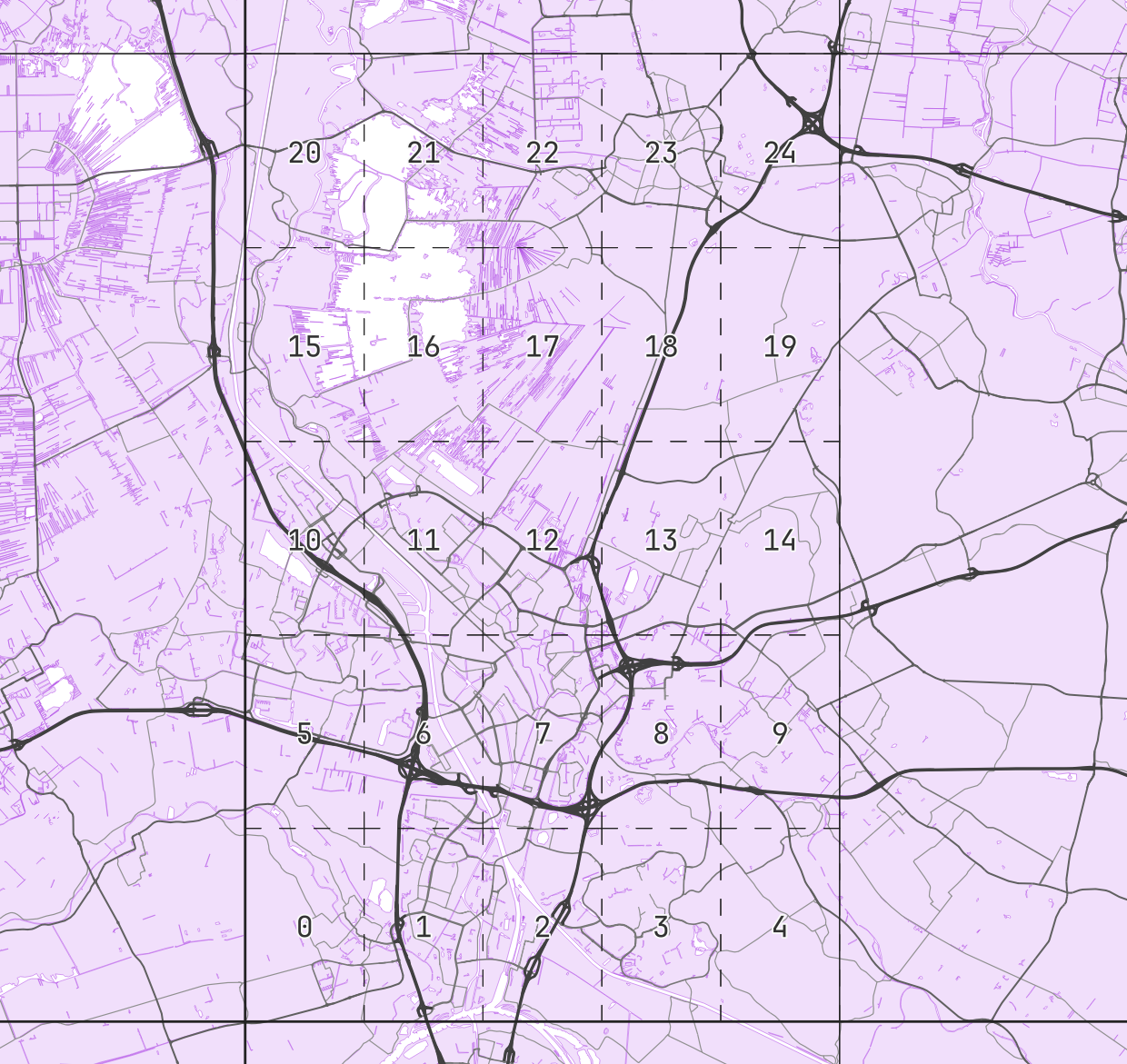
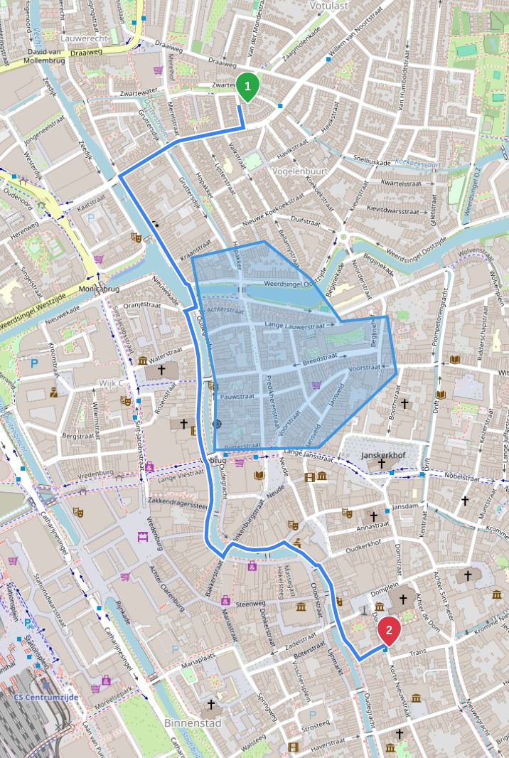
This takes care of the tile-crossing edge problem: for an edge that runs through multiple bins, we just store its ID in every bin’s list. Let’s look at an example from a bin south of Utrecht’s city center:

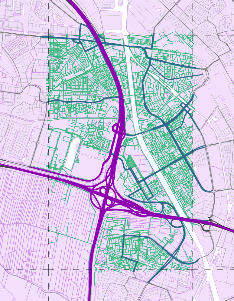
As you can see on the borders, edges spilling over into neighboring bins are stored here as well, regardless of the hierarchy level they are on.

So to recap: instead of brute forcing its way through every edge on the entire globe, Valhalla’s grid structure helps it focus on only a few kilometers of search space. But as the above image shows, even a square of a few kilometers in size can contain tens of thousands of edges. What can we build on top of that to help the location search discard even more edges early on, without having to evaluate their exact distances to input points?

Bounding Circles to the Rescue

Almost any approach to spatial indexing involves storing some kind of bounding geometry. Most commonly, the axis aligned bounding box is used. It is a very simple geometry (stored as a minimum point and a maximum point) defined as the smallest possible rectangle that encloses all of a geometry’s points, and helps quickly determine whether the actual underlying geometry is even remotely close to our input. But for Valhalla, disk space is precious (the planet-wide graph already consumes almost 100 GB), and storing two full coordinates per edge would be prohibitively expensive at this scale: in full double precision, a bounding box for each edge would cost us roughly ~30 GB!

So our solution has to somehow minimize the amount of space needed per edge bounding geometry, while still being useful. Luckily there are a few things we can do. The first is to store a circle instead of a box since circles can be expressed in 3 rather than 4 numbers: longitude, latitude and radius. This saves us space at the expense of precision (imagine the bounding box vs. the bounding circle of a straight edge running north). The second thing we can do is quantize these three numbers so they fit in less space. Here we can use some clever tricks.

Quantizing the center coordinate

The smart thing to do would be to store our bounding circles as an array running parallel to our bins’ edge ID arrays. That way, we can iterate both simultaneously and have quick access to the bounding circle given an edge ID. And this gives us even more: at the time we’re looking at a circle, we know which bin it’s in. This is great news, because rather than storing the circle center as absolute global longitude and latitude, we can store it as coordinates relative to the bin center. And if we cap the maximum allowed radius of any circle (more on that in a bit), we can define the full extent of our bin-local coordinate system as the bin size plus twice the maximum valid radius.

Quantizing the radius

Here’s a fact: most edges are short. But some edges are really long. Hence, most bounding circles will have small radii, while only a handful will have very large ones. The global distribution of minimum bounding circles’ radii shows this:

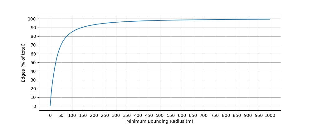
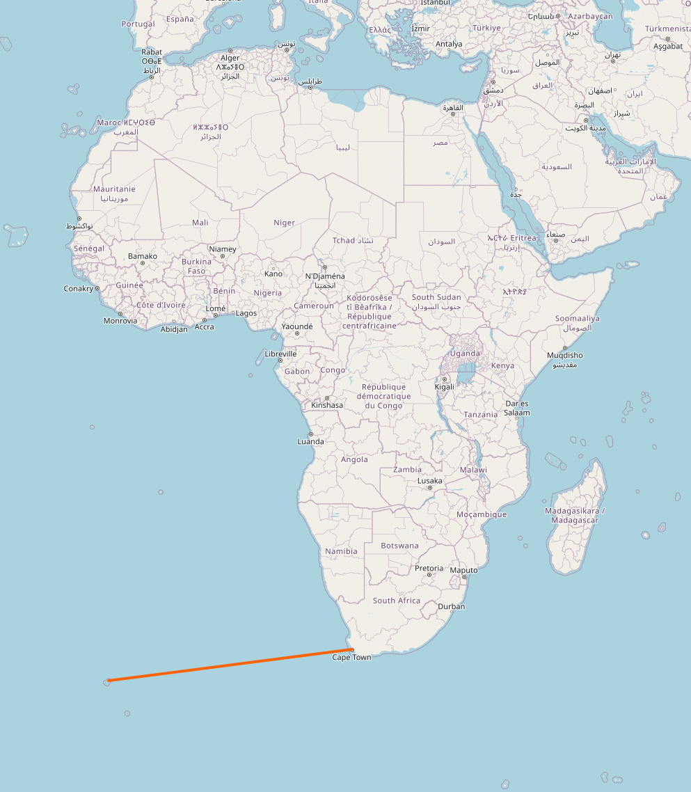
You might say “Come on, a 1000 meters, that’s not too bad”, just to read the above caption again and see it’s cut off at the 99.97% percentile. You look up the longest routable way in entire OpenStreetMap, and find this ferry line running from Cape Town, SA to Tristan da Cunha, at roughly 3000 km. If we were to extent our range of valid radii to that value, not only would we sacrifice precision in the much more common low value range, we would also not gain anything in terms of performance: most bins that intersect this edge would be covered completely by the bounding circle formed for the edge, so any point within the bin would also be inside the circle, giving us little possibility of rejecting the edge early on in our search.

So it only does it make sense to pick a sensible maximum value; for edges whose bounding circle exceeds this maximum, we can come up with a special value indicating the circle is invalid. This tells our search algorithm to simply go check the full geometry in these rare cases. Looking at the distribution of radii again, we see it’s heavily skewed towards the left: more than 80% of radii are below 100 meters. Hence, the smart move here would be to use a non-linear quantization scheme to fit our non-linear distribution. The easiest way to do this in practice is to not store radii on disk at all: rather, we store a fixed size list of radii in our code, and only write the indices to that list to disk.

Finding the best middle ground

We know more or less how we want to quantize our circles, and how to write them to disk. Now we need to define the size in which we want to fit the center coordinates and the radius. I picked an overall size of 4 bytes (32 bits) per circle. This would add an additional 8 GB to the planet-wide graph, an increase of just under 10%. Per coordinate, I choose 13 bits (=8192 values), leaving 6 bits, or 64 values, for the radii. The highest radius is defined at 2500 meters (so the largest circle covers roughly half a bin at zero latitude). Around the equator, this gives a coordinate precision of ~1.3 meters (defined as ((bin_size) * meters_per_latitude_degree + largest_allowed_radius) / 8192), decreasing as we move towards the poles.

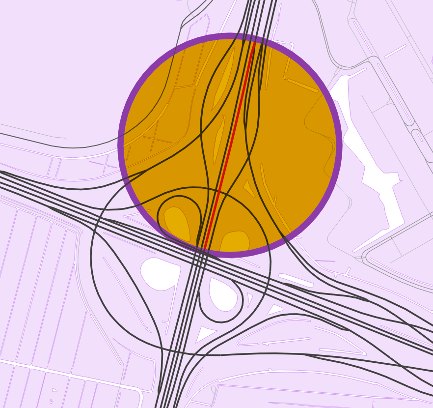
The final set of radii was, after a lot of experimentation, not picked algorithmically. I tried out various approaches, such as k-means clustering, to find the set of radii that minimizes the sum of errors between the raw radii and its quantized variants. In the end, the combination of radii that performed best in the benchmarks was one I had kind of put together following a lot of trial and error, roughly following the radii distribution so that most radii are below 100m. And as you can see in the example above, the quantization error even for edges with a minimum bounding circle radius >100m is still very small.

Note: You might be asking “why store the radii in meters if Valhalla only ever uses spherical lat/lon coordinates?” It is true that if we stored radii in relative degrees, we could save a few calculations when measuring our candidate’s distance to an edge’s bounding circle. The answer why we use meters is that the actual unit size of a degree longitude decreases as we move toward the poles. Simply put, 0.05° longitude equal about ~5.5 kilometers at the equator, but in Longyearbyen, one of the permanent human settlements closest to the poles at about 78° latitude, 0.05° longitude amount to only 1.1 kilometers, but 0.05° in latitude change is still ~5.5 kilometers! This just complicates things! The extra meters to degree conversion is cheap enough and makes our lives easier.

Putting it to use

Finally, we have our spatial index. At just 4 bytes per entry, which is half of what the edge IDs themselves occupy in the bins, we’ve just added about ~8GB worth of bounding circles to the planet graph. Now we can use it! Before evaluating an edge that’s in a close by bin, we can simply look at its bounding circle and try to reject it based on

1. whether the user specified a search radius and the bounding circle is outside of it
2. whether our current best candidate is closer to the location than the closest point in the bounding circle

I benchmarked Valhalla’s location search using lots and lots of GPS data from cycling trips around the Netherlands, and the results look promising:

• the smaller the number of locations, the greater the difference: with bounding circles, searching with a single location is a couple of hundred times faster than without bounding circles, with up to 5 locations at once, it’s still about 10 times faster
• eventually, for large numbers of locations, it converges to being about 2 times (when the user did not provide a radius, meaning the single best candidate is found) to 3 times faster (with a fixed radius specified, meaning any edge inside the radius is returned)

The interesting use case is of course the one including many locations: for a few locations (such as for point-to-point routing), the algorithm is already fast and the actual path finding algorithm already takes up a lot more processing time than the location search. But there are many more cases where this index will benefit Valhalla.

Further uses

For a 2-3x speedup of the location search, increasing the tile size by just under 10% sounds like a lot, but the optimization opportunities don’t stop here: Valhalla has to perform spatial candidate searches well beyond finding candidate edges for its routing. Here are some of them.

Excluding entire areas in path finding

One of Valhalla’s most interesting features is that it lets users specify arbitrary polygon rings, excluding any intersecting edges from the final path. This feature is notoriously slow on larger inputs, because it does not perform any early rejection on edge candidates in a bin intersecting a ring. So while small rings with few vertices are noticeably fast, the performance steeply drops once the overall vertex count increases. And this was precisely my motivation to introduce better spatial indexing in the first place.

With the bounding circles, we can quickly reject a good amount of edges and avoid a lot of expensive intersection tests. Just like the location search, the performance improvement depends on the input. But here is where the bounding circles really shine: for a few large polygons, there is a ~20-30x speed up, while for lots of small polygons, I observed a >200x speed up, cutting the processing time from ~10s to tens of milliseconds. As this was my principal motivation to get started on this feature, seeing these numbers made me really happy.

Dynamic vector tile generation

Valhalla’s new /tile end point offers users to visualize the road network using MapBox Vector Tiles (MVT), optionally with all sorts of information on live traffic, access restrictions and more. With the bounding circles, dynamically collecting all edges intersecting a vector tile boundary becomes much faster, especially on high zoom levels, where most edges in a given bin will be outside of the tile box. On zoom level 11, I measured a ~1.5x speed up compared to before, while on zoom level 14, that value was closer to 4x on a warm tile cache.

Map Matching (TBD)

The original reason Kevin had the initial idea for bounding circles was to use the location search used for routing in map matching. Currently, Valhalla’s map matching module, meili, uses its own simplified location search. This focuses on low latency and sacrifices two aspects in order to obtain it:

1. RAM: each worker uses its own in-memory location cache, which can take up lots of space, especially when running many worker instances on the same machine
2. Location search goodies: Valhalla’s default location search, loki, has lots of features that are useful for location filtering, which meili’s search compromises on.

Getting rid of meili’s search would require loki’s search to become much faster, and the bounding circles may just have pushed it into the realm of feasibility. I haven’t gotten around to replacing meili’s search yet, but it’s on my list. If anyone is interested in better location filtering for map matching, feel free to reach to me via chrstn at <this_domain> dot de.

Wrapping up

And that’s it, this blog post ended up being longer than I anticipated, but it’s a feature I have enjoyed working on for quite some time, and I am quite proud of the outcome. Huge thanks to Kevin for the original idea, and inspiration and guidance along the way!